Continue Testing DCS and SF
City 1000
The first dataset that we will look at is the commonly used city10000. This is a simulated dataset, which was original pose graph can be seen below.
Pose Graph for City 10,000
Interestingly, the Levenberg–Marquardt least-squares would not work on this specific dataset. So, for this dataset, the Gauss–Newton implementation was used. A side-by-side comparison of the L-M and G-N algorithms attempting to optimize the city10000 graph is shown below ( Gauss-Newton implementation is shown on the right ).
Using the initial error free pose graph shown above, multiple false constraints were added to evaluate the performance of the robust optimization scheme. As a reference, the results for traditional $L^2$ optimization when 10 false constraints are present is $\mathcal{X}^2$ = 21634.

CSAIL
This dataset is built from raw data acquired at the MIT CSAIL building (the relative pose measurements are also available here )

Inital Pose Graph for CSAIL
Again, using the initial error free pose graph shown above, multiple false constraints were added to evaluate the performance of the robust optimization scheme. The results for DCS and switch factors are shown below.

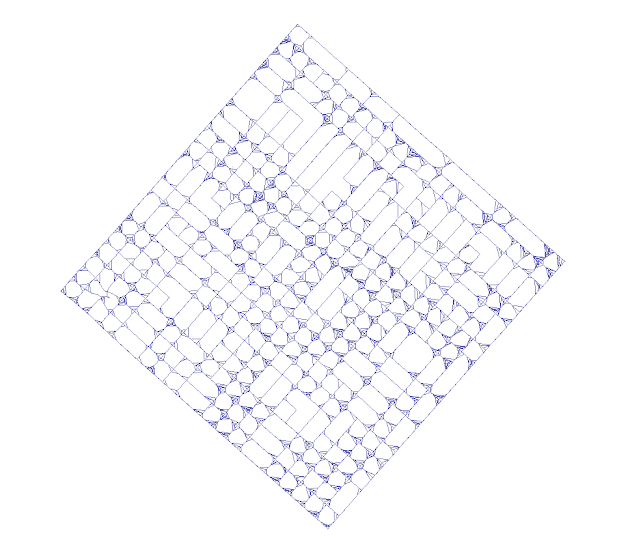
Freiburg Building
This pose graph is generated from raw data acquired at the Freiburg Building (the relative pose measurements are also available here )

Inital Pose Graph for FR079
Faults were added to the fault free graph in the same manner as state before. The results for DCS and switch factors are shown below.

Freiburg Clinic

Inital Pose Graph for Freiburg Clinic